Introduction

This blog aims to provide facts about SPH convergence. Everything here is from a single paper by Quinlan et.al. (Quinlan & Cummins, 2006), which in my opinion is one of the most important papers in the field of SPH. I focus more on the implications of Quinlan’s study rather than the mathematical derivations he uses to prove his point. Thus, this blog post might be useful for practitioners of SPH, who want to know what parameters affect convergence and how they affect it, rather than mathematicians who want the proof of how the parameters affect convergence. That being said, I try to state the assumptions and gotcha’s on what these general statements about SPH convergence are based. The blog assumes basic knowledge of SPH and so none is provided here.

Note: If you are interested in reading just four lines and still getting some insight on the topic, read the Give me four points I should remember forever section.

Why is SPH convergence different and worth studying?

Most mesh-based methods (like FEM, FVM, etc.) converge to the exact solution of the PDE as the mesh is refined. If you have used any of these methods, you would probably have reduced the mesh size to at least a point where the obtained solution does not change much with further refinement. However, SPH is different in that it is a “two-stage” method involving two forms of errors that counteract each other. Let me explain -

• Smoothing Error: Consider the Dirac delta identity, which evaluates a value of any function at a point \(r\) by summing the values of the function at all points \(r'\) in the domain, given by

  \[f(r) = \int_{-\infty}^{\infty} f(r') \delta(r-r') dr'\]

  SPH replaces the Dirac delta function (which is impossible to represent in a computer) with a kernel function \(W\) (think of a Gaussian function which tends to the Dirac delta function as the width of the Gaussian tends to zero) to get

  \[f(r) = \int_{-\infty}^{\infty} f(r') W(r-r',h) dr'\]

  The \(h\) here defines a cut-off radius for the kernel function. Usually, beyond \(2h\) the kernel function is zero and those particles are not considered in the integral (so now think of a truncated Gaussian). Replacing the Dirac Delta function with a kernel function introduces a smoothing error, which as you would guess depends on h (the smoothing length). Note that the Dirac Delta function has a \(h = 0\).

• Truncation Error: The integral is then approximated by a summation over the discrete points in the domain. Thus, \(f(r)\) becomes

  \[f(r) = \sum_{j=1}^{N} f(r_j) W(r-r_j,h) V_j\]

  where \(V_j\) is the volume of the particle at \(r_j\) and \(N\) are the neighbors of the particle at \(r\) (within \(2h\)). This introduces a truncation error, which, as you would guess, depends on the number of particles in the kernel support (\(N\))and how these particles divide the kernel volume (\(V_j\)) (whether they are uniformly distributed or not).

We now have a dilemma - if we want to reduce the smoothing error, we need to reduce \(h\). However, if we reduce \(h\) and keep our domain discretization the same (defined by the initial spacing between the particles \(\Delta x\)), we will keep reducing the number of particles in the kernel support (\(N\)) thus increasing discretization error. Else, like in mesh-based methods, if we keep reducing the particle spacing \(\Delta x\) and keep \(h\) constant, then the discretization error will decrease, but the smoothing error will stay the same, and we will hit a wall. So what do we do? Listen to Quinlan et.al.

Quinlan’s Study

(Quinlan & Cummins, 2006) tells us error trends while evaluating the gradient of a function \(f(r)\) using SPH. Note, in the above section we only discussed the approximations for the value of a function, not its gradient. It turns out however that the same formulas hold for the gradient of the function, where the gradient ends up on the analytically defined kernel function \(W\) (pretty neat right?) -

\[\nabla f(r) = \sum_{j=1}^{N} f(r_j) \nabla W(r-r_j,h) V_j\]

The error trends are estimated both analytically and empirically using numerical experiments. The investigations are done both for a uniform and non-uniform particle distribution. Further, the study is also extended to kernels (or modifications of kernels) that are first order consistent (more on this later).

Notational conventions and assumptions

Before we start, lets ensure we have the same understanding of the greek letters. In my world, \(\Delta x\) is the initial spacing between the particles that discretize the domain (these are the “SPH markers”), \(h\) is the smoothing length of the kernel function, \(N\) is the number of particles in the kernel support, \(V_j\) is the volume of the particle at \(r_j\) and \(W\) is the kernel function. Further, the kernel is assumed to have compact support, i.e. \(W(r-r_j,h) = 0\) for \(|r-r_j| > 2h\). Throughout the study, the data function of interest (the one whose gradients we are approximating using SPH) is assumed to be \(f(r) = A(x) = A_0 \sin(2\pi x / \lambda)\). The \(\lambda\) provides the characteristic length scale of the data function being approximated. The analytical error analysis is done predominantly in 1D, however, the 1D results carry over to 3D (verified empirically).

We will see that our error trends largely depend on the boundary smoothness of the kernel which is defined as the highest integer \(\beta\) such that the \(\beta\)th derivative of the kernel function and all lower derivatives are zero at the edges of the compact support (what a weird definition right?). The two commonly used kernels, the cubic spline and Wendland’s C4 kernel, are both \(\beta = 2\).

Case 1: Uniform Particle Distribution without First Order Consistency

The total error in approximating the gradient of a function \(f(r)\) using SPH without first order consistency and for a uniform particle distribution is \(O\left[h^2 + \left(\frac{\Delta x}{h}\right)^{\frac{\beta}{2}}\right]\)

If you wish to know how, look at Quinlan’s paper.

What are the implications of this?

Quinlan provides analytical and empirical results for the error trends with various values of \(h\) and \(\frac{\Delta x}{h}\). \(h\) is normalized with the characteristic length scale \(\lambda\) (remember our data function is a sine function with wavelength \(\lambda\)).

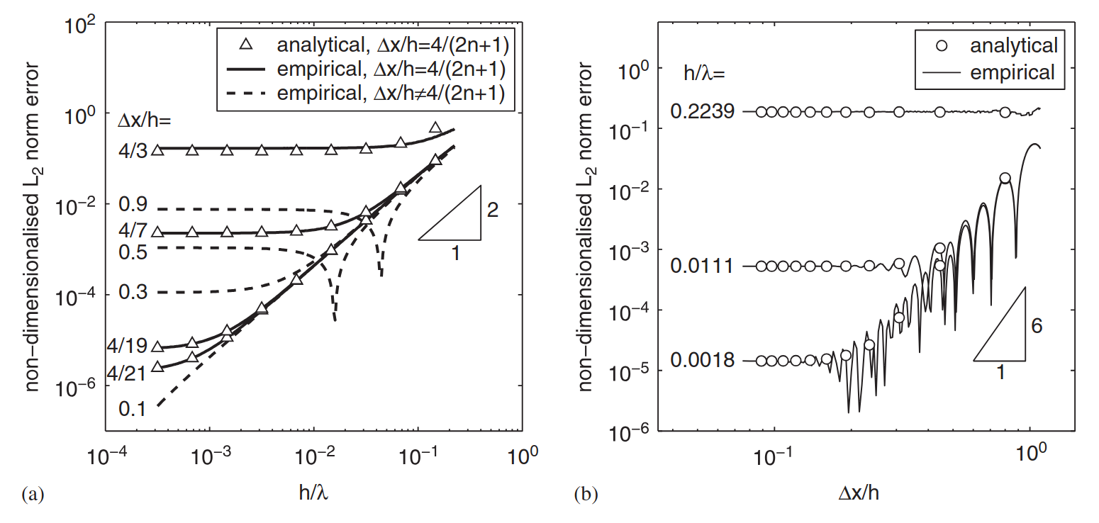
Lets start with Figure 1(a). The x-axis is normalized \(h\) whereas the y axis is the L2 norm of the error. There are many curves, each representing different values of \(\frac{\Delta x}{h}\).

• You can see that some lines are dotted - these are lines where the equation \(\frac{\Delta x}{h} = \frac{4}{2n+1}\), where \(n > 0\) is an integer, does not hold. As you can see that the dotted line is not an analytical result - this is because the analysis in the paper only holds for \(\frac{\Delta x}{h} = \frac{4}{2n+1}\). Only when this equation holds, the volumes of the particles (in 1D this is \(\Delta x\)) fill the kernel support of diameter \(4h\), without gaps or overlaps. This is interesting because you can see that the dotted lines have a weird drop to a minima. This means that there are “special” \(\frac{h}{\lambda}\) at which the error is minimum. But why? Unfortunately, my guess is good as yours and Quinlans.
• Now, looking at the solid lines, you can see the error reduces quadratically with \(h\) (see the tiny triangle showing the slope for quadratic convergence). This is expected because the smoothing error, which is one component of the total error is \(O(h^2)\).However the error drop hits a wall! This is when the discretization error dominates! Additionally, notice that the higher the value of \(\frac{\Delta x}{h}\), the earlier (larger \(\frac{h}{\lambda}\)) the discretization error starts dominating.

This means that if I were to keep \(\frac{\Delta x}{h}\) constant and reduce \(h\) (note, this is exactly the same as reducing \(\Delta x\) and keeping \(\frac{\Delta x}{h}\) constant), the error would reduce quadratically with \(h\) until I hit the discretization error wall.

In most commercial SPH codes, the user is provided an option to set \(\Delta x\) and the ratio \(\frac{\Delta x}{h}\). Thus, it is very easy to fall into the trap of thinking that reducing \(\Delta x\) and keeping the same \(\frac{\Delta x}{h}\) will reduce the error. Such an approach also works with other methods like FEM,FVM where one would just refine the mesh and the error would reduce. However, for SPH, one cannot expect the error to reduce just by reducing \(\Delta x\) and keeping the same \(\frac{\Delta x}{h}\).

Now, looking at Figure 1(b), the x-axis is now \(\frac{\Delta x}{h}\) with the y-axis being the L2 norm of the error. Each of the solid lines corresponds to a different value of \(\frac{h}{\lambda}\).

• As you can see from looking at the tiny triangle, the error now reduces as \(O(\frac{\Delta x}{h})^{6}\). This is what we expect with a kernel function of \(\beta = 4\), which is what is used.
• Interestingly, for the empirical results, the error trends again have a bunch of local minima. Quinlan claims that this these “correspond to points where the error changes sign”. Although I do not understand what he means by this.

Thus if I were to reduce \(\frac{\Delta x}{h}\) and keep \(h\) constant, at some point I would hit the smoothing error wall!

Case 2: Arbitrary Particle Distribution without First Order Consistency

In a real-world simulation, it is rarely the case that the SPH particle distribution remains nice and uniform. Its thus interesting to understand what happens to SPH error trends when the particle distribution is messy. In Quinlan’s study, arbitrary particle distributions are generated by applying a normally distributed perturbation with standard deviation \(\sigma\) to the particle positions.

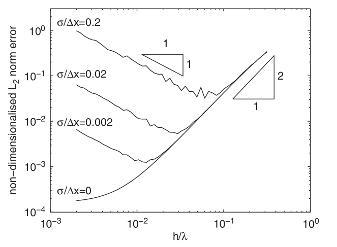
Oh boy, the curves are going upwards! Lets look at Figure 2 more closely. First, \(\frac{\Delta x}{h}\) is fixed at 0.364 (a reasonable value) and \(\frac{h}{\lambda}\) is varied along the x-axis. There are 4 solid lines, each corresponding to different degrees of perturbation, parameterized by a normalized standard deviation \(\frac{\sigma}{\Delta x}\).

• Like in Figure 1(a), with reducing \(h\), the error reduces quadratically until the Discretization Error Wall is hit.
• However, things get funky here. First, if there is any perturbation (\(\frac{\sigma}{\Delta x} > 0\)), the error diverges! Additionally, the error divergence starts earlier (at a higher \(\frac{h}{\lambda}\)) for more perturbed distributions. The rate of divergence remains the same (linear).

This means that if I am doing any kind of SPH simulation where the particles all don’t move nicely and uniformly (the case most of the time) and I use my muscle memory from FEM and FVM like methods to only decrease \(\Delta x\) and keep \(\frac{\Delta x}{h}\) constant, I will not just not converge, but I will diverge! In other words, when \(h\) is large, the error is second order in \(h\) and when \(h\) is small, the error is of order \(h^{-1}\) (divergence!).

Can we get error reduction if we keep \(h\) fixed and vary \(\frac{\Delta x}{h}\)?

Quinlan analyzed for both a small value of \(\frac{h}{\lambda} = 0.022\) (Fig. 3(a)) and a large value of \(\frac{h}{\lambda} = 0.2\) (Fig. 3(b)).

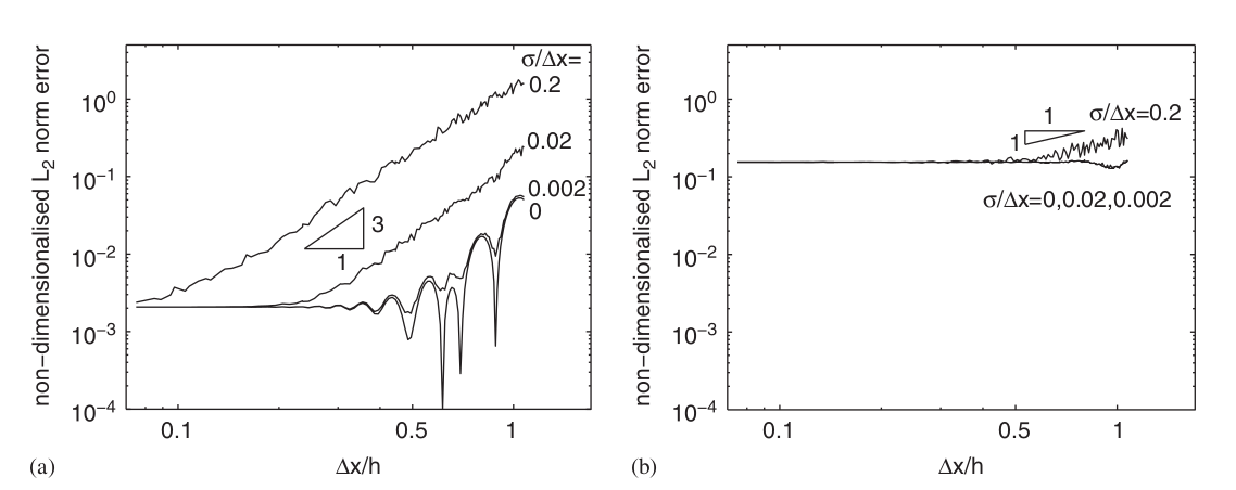
• Figure 3(b) shows that when \(h\) is large, you hit the smoothing error wall pretty early. Additionally, we see that the error decreases with only first order for high perturbation and does not decrease at all for low perturbation (you can also see that the low perturbation case matches Fig. 1(b)).
• However, when \(h\) is small, as in Figure 3(a), we find the error reducing cubically until the smoothing error terms dominate. Interestingly, we can see that this is the case even for large perturbations and that there is no divergence!
• Notice that in this case the error trends have no dependence with the boundary smoothness of the kernel \(\beta\).

What this means is that if I know that my particle distribution is not going to nice and uniform, irrespective of the kernel I choose, I should start with a small \(h\) (relative to the characteristic length scale of the problem) and then keep reducing \(\frac{\Delta x}{h}\). In this case, I can expect the error to decrease cubically until the smoothing error terms start dominating.

Case 3 Arbitrary Particle Distribution with First Order Consistency

The natural question to ask is, can we gaurentee convergence, even with keeping \(\frac{\Delta x}{h}\) constant? Interestingly, the answer is yes and the mechanism of doing so is to use a kernel that is first order consistent.
Very briefly, a kernel is said to be first order consistent if it exactly recovers the gradient of a linear function. Thus, if you look at the error terms from Quinlan’s paper, you will find that they do not have any terms with coefficients \(A\) of \(A'\) (where A is the data function) for an SPH approximation with a first order consistent kernel. This means that if \(A\) were linear, the error would be zero (since \(A''\) and beyond are zero anyways for a linear function).
But what does this mean for higher order of data functions? Also how does my error behave when I have arbitrary particle distributions with first order consistency? Do I still have divergence? Lets look at the data Quainlan presents:

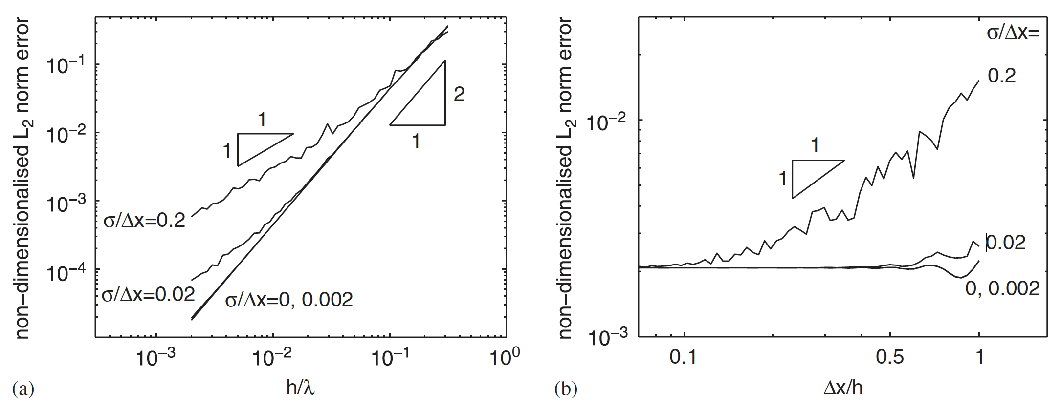
• Figure 4(a) is a direct comparison with Figure 2, where in the former, consistent discretization is used and in the latter it is not. Additionally, in Figure 4(a) the \(\frac{\Delta x}{h}\) is fixed at a higher value (0.7 - meaning less computationally expensive) than in Figure 2 (0.364 - meaning more computationally expensive). However, surprisingly, there is no divergence in Figure 4(a) even for high perturbations!

This means that if I use kernels that is at least first order consistent, I can keep \(\frac{\Delta x}{h}\) constant and reduce \(h\) (or \(\Delta x\)) and still expect the error to decrease quadratically for small perturbations and linearly for large perturbations. This is a much better result than when I don’t use first order consistency where I would see divergence at high perturbations. Thus using first order consistent kernels greatly improves robustness to particle perturbations.

• Figure 4(b) is a direct comparison with Figure 3(a), where the former uses first order consistent kernels and the latter does not. In this case both plots also use the same \(\frac{h}{\lambda}\) (0.022). Here we can see that with consistent discretization the error starts of at a lower value (for example at \(\frac{\Delta x}{h} = 1\) and highest perturbation, the error with consistent discretization is \(10^{-2}\) whereas without it is \(10^{0}\)). However, the error decays linearly with consistent discretization and cubically without it. But if you look closely, for a particular \(\frac{\Delta x}{h}\), and this is true at all values of \(\frac{\Delta x}{h}\), the error with consistent discretization is lower than without it.

This again shows the power of using first order consistent kernels. You are always going to end up with a lower error with it, even at higher perturbations.

Not all is rosy as using first order consistent kernels is associated with a computational cost. It would be interesting to study if, due to better error trends, one can achieve computational savings and better accuracy using first order consistent kernels.

I don’t want to deal with consistent discretization, is there still hope for guaranteed convergence?

Consistent discretization adds complexity and computational cost to the SPH method. Additionally, in Figure 3, we saw that there is hope if we are very careful with how we vary \(h\) and \(\frac{\Delta x}{h}\). Quinlan did some nice analysis on this. Consider the below empirical results:

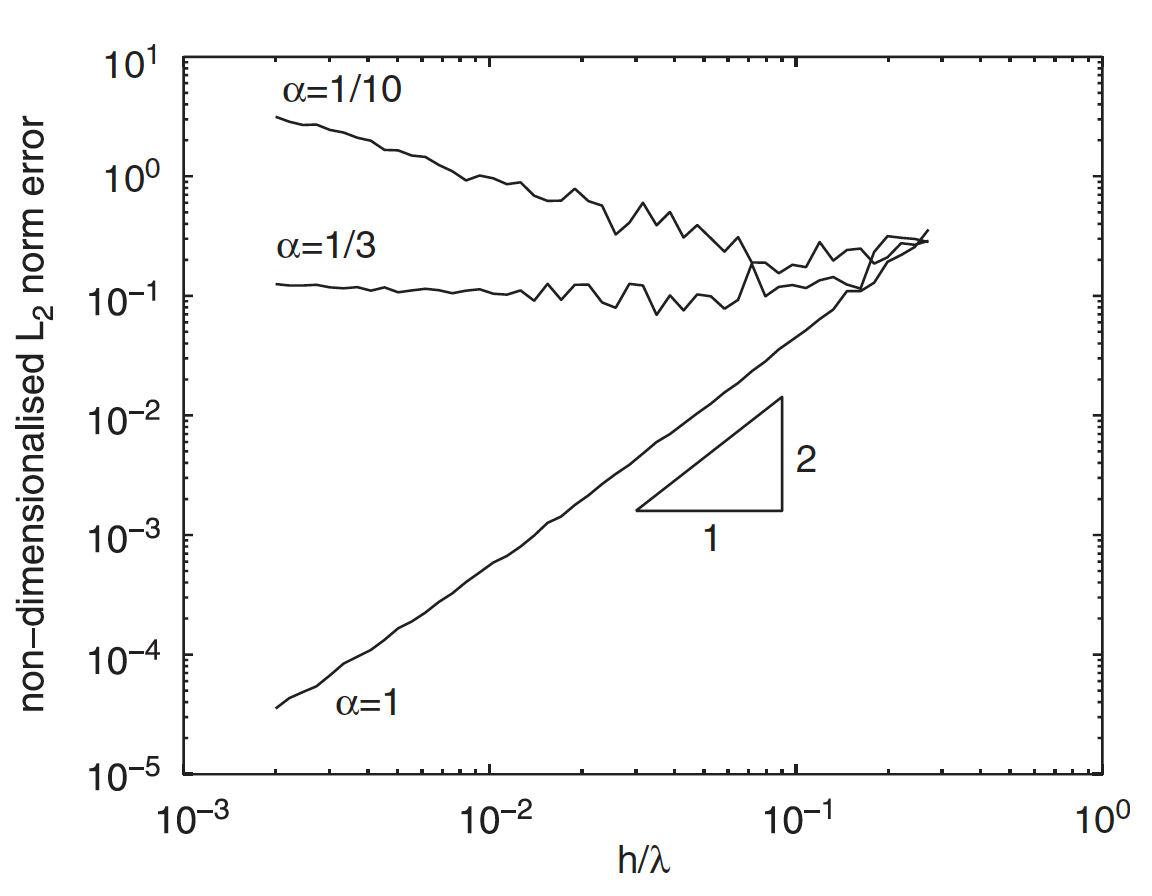
The \(\alpha\) in the plot indicates how much you would need to change \(\Delta x\) when you change \(h\). For instance, if you pick \(\alpha = 1\), then you need \(\frac{\Delta x}{h^2} \propto 1\), which means if you were to reduce \(h\) by a factor of 2, you would need to reduce \(\Delta x\) by a factor of 4. If you do this, then you will be guaranteed quadratic convergence even without consistent discretization (note the results are for high perturbation \(\frac{\sigma}{\Delta x} = 0.2\))! However, if you where to pick any \(\lambda < \frac{1}{3}\), you would get divergence as you reduce \(h\).

Give me four points I should remember forever

• Use first order consistent discretization if you don’t want to worry about convergence.
• If you don’t use first order consistent discretization, then you need to be very careful with how you vary \(h\) and \(\Delta x\) to ensure convergence.
• If you don’t use first order consistent discretization, then make sure that when you reduce \(h\) by a factor of \(k\), you at least reduce \(\Delta x\) by a factor of \(k^{\frac{4}{3}}\).
• Use smooth kernels with high boundary smoothness - you will hit the discretization error wall later.

What next?

I think it would be very interesting to bring in computational effort into this analysis. For instance, it would be interesting to compare the computational cost of doing consistent discretization and seeing if that is offset by not having to use a very small \(\frac{\Delta x}{h}\) (remember, a smaller \(\frac{\Delta x}{h}\) means more particles in the kernel support and more computational effort).

References

2006

1. Truncation Error in Mesh-Free Particle Methods

   Nathan J. Quinlan , and Eugene J. Cummins

   International Journal for Numerical Methods in Engineering, 2006